What Is a Bonding Curve in Crypto and How Does It Work?

What Is a Bonding Curve?

Programs and platforms built on blockchains are continuously seeking ways to enhance decentralization and automation. In recent years, many protocol ecosystems still require external entities such as exchanges to carry out some of their functions. By employing smart contracts, blockchains have been able to move many functions into a more automated and decentralized sphere. Moreover, increased use of mathematical algorithms is allowing for a broader range of transactions to be carried out without any human or external interference. This progress is enabling blockchain protocol ecosystems to become increasingly independent, decentralized, and automated. One mathematical concept that is making significant waves in this space is an automated market maker (AMM) known as a bonding curve.

Initially conceived by Simon de la Rouviere in 2017, a bonding curve is a mathematical concept that can be built into platforms and applications to calculate a token's value as determined by its supply. The fundamental principle is straightforward yet powerful: as more tokens are purchased, the price increases according to a predetermined mathematical formula. Investors buy tokens according to the price listed on the bonding curve, in exchange for collateral in fiat currencies or other cryptocurrencies, such as Bitcoin (BTC) and Ethereum (ETH). The bonding curve's value estimate of the token is taken when investors buy tokens (where they are minted) and when they sell tokens (where they are burned). As these bonding curve tokens are minted and burned, the supply changes, which will in turn be reflected in the value listed by the bonding curve.

Bonding curves serve multiple critical functions in the cryptocurrency ecosystem:

Improving Valuations: Bonding curves are transparent as they are built into blockchains, and they are predictable and accurate as they are constructed using mathematical formulas. This transparency eliminates the opacity often associated with traditional valuation methods. Bonding curves also provide a dynamic approach to calculating cryptocurrency values, as they take ecosystem growth into consideration. A bonding curve recognizes that as an ecosystem grows, so does the amount of that ecosystem's token, and subsequently so does its value. This creates a self-reinforcing mechanism where growth begets value, and value attracts further growth.

Pre-setting How Token Value Will Increase or Decrease: A bonding curve establishes that token and coin prices will change with their supply, either decreasing or increasing, thereby creating a continuous token model. This predictability is valuable for both developers and investors. If a developer wants to take more control over this aspect, they can choose a specific bonding curve shape, which will determine how much a token's value will increase based on supply. Different curve shapes can incentivize different behaviors, from rewarding early adopters to maintaining steady growth over time.

Removing the Need for Exchanges: As a fully automated market maker (AMM), bonding curves not only allow for the calculation of a token's price but also enable transactions directly. The mathematical algorithm estimates the cost of the token, which it shows to the investor. After this, the investor can simply buy or sell their tokens right there, without needing to list on centralized exchanges or wait for order matching. This function is particularly exciting, as it moves cryptocurrency further away from centralization and reduces dependency on third-party intermediaries, thereby enhancing security and reducing costs.

Allowing for Multiple Tokens in One Ecosystem: Another powerful function of a bonding curve is that by minting its own tokens, it can allow for multiple tokens to be used within one ecosystem. A developer can build multiple bonding curves into the ecosystem, thereby allowing for different tokens to be used for different projects, according to the functionality that the developer wants. This allows for greater versatility as different tokens can be used across different blockchains, depending on the usage of the token and the smart contracts or two-way pegs that connect the blockchains. This multi-token approach enables more sophisticated economic models within decentralized applications.

How Does a Bonding Curve Work?

Understanding the mechanics of a bonding curve requires examining a practical example. A simple linear bonding curve states that x = y, which is to say, token supply = token value. This means that token number 10 will cost $10 and token number 20 will cost $20. However, this does not mean that if an individual buys 10 tokens, they will pay $10. The calculation is more nuanced.

Token 1 will cost $1, token 2 will cost $2, token 3 will cost $3, and so on. Thus, if an individual wants to buy 10 tokens, they will have to pay the price of each of those 10 tokens, which would be $1+$2+$3+$4+$5+$6+$7+$8+$9+$10, totaling a cost of $55. If an individual wants to buy 10 coins, but 10 have already been purchased, then the individual in question would buy from token 11 to token 20. This means that they would pay $11+$12+$13+$14+$15+$16+$17+$18+$19+$20, totaling $155. Thus, this type of linear bonding curve gives higher profit potential to early investors, creating a natural incentive for early participation.

The selling mechanism works in reverse. If these investors were to sell, the early investor would make a larger profit. The early investor bought 10 tokens for $55, but with the subsequent investment from the second individual, the token value went up. This means that the first investor can sell at the new, higher value. For example, if they sell their 10 tokens (tokens 1-10) after the second investor has purchased, they would receive $1+$2+$3+$4+$5+$6+$7+$8+$9+$10 = $55 back, but the actual market value of those positions has increased.

Once the first investor sells their tokens, these are burned, which means that there are fewer tokens in circulation. The supply has therefore decreased, meaning that the value has too. The second investor who bought their 10 tokens for $155 would therefore lose money if they sold immediately at this point, as the price would have reverted to a lower level due to the reduced supply.

A bonding curve allows for investors to buy or sell their tokens at any point in time, providing continuous liquidity. However, as with any investment, this could result in profit or loss depending on the market dynamics and timing. When building their programs, developers can control how much profit or loss an investor will make depending at which point in the bonding curve they make their transaction. This is done by choosing a particular shape for the bonding curve, which we will explore in the next section.

Applications of Bonding Curves in Crypto

Bonding curves first gained attention in the late 2010s when projects looked for new ways to raise funds and bootstrap markets. Since then, they have been applied in various contexts across the cryptocurrency ecosystem, demonstrating their versatility and utility.

Token Sales and Initial Offerings: A bonding curve allows continuous token sales, differentiating from traditional ICOs where a fixed number of tokens are sold at a set price. This continuous model offers several advantages. Early supporters can buy tokens at lower prices, with prices rising as demand increases, linking funding directly to interest and creating a more organic growth pattern. For instance, Fairmint's Continuous Organization model lets companies raise funds through a bonding curve, providing ongoing liquidity for investors. Another notable example is Pump.fun, which creates a bonding curve for meme coins on Solana, ensuring liquidity and smooth price increases without needing exchange listings. This approach has democratized token launches, making them accessible to projects of all sizes.

Automated Market Makers: Decentralized exchange platforms have successfully implemented bonding curve principles for trading pairs. Uniswap's constant product formula (x * y = k) functions as a type of bonding curve, enabling automated trading without order books. Similarly, Curve Finance optimizes for stablecoin trading with a specialized flat curve designed to minimize slippage for assets that should maintain similar values. These DEXs showcase the remarkable success of bonding curve mechanisms in offering deep liquidity and enabling substantial trading volumes without intermediaries, processing billions of dollars in daily trading volume.

Stablecoins: Some algorithmic stablecoins have employed bonding curve logic to maintain pegs by adjusting supply based on demand. The mechanism works by expanding supply when price exceeds the peg and contracting it when price falls below. However, this approach can lead to significant risks, as seen in TerraUSD's catastrophic loss of its peg in 2022, which highlighted the challenges of purely algorithmic stabilization. Other projects, such as Ampleforth, use similar supply adjustments with elastic supply mechanisms to target price maintenance, though with varying degrees of success. These examples demonstrate both the potential and limitations of bonding curve applications in stablecoin design.

Governance and DAO Tokens: Bonding curves can also effectively fund Decentralized Autonomous Organizations (DAOs). Individuals pay into the curve for governance tokens, with prices rising as more participants join. This creates an evolving membership model where the community grows organically. Exiting members can sell back to the curve, providing liquidity while ensuring that remaining participants maintain value. Projects like DAOstack and CommonStack have utilized this method to manage member dynamics while maintaining value for remaining participants, creating sustainable funding models for decentralized governance structures.

NFTs and Digital Art: In the NFT space, bonding curves have been used to gradually increase prices as more editions are sold. This model incentivizes early collectors with lower prices while ensuring that creators capture increasing value as demand grows. However, the application has faced some criticism in certain implementations, particularly when the pricing mechanism is not clearly communicated to buyers or when it creates excessive speculation rather than genuine collecting interest.

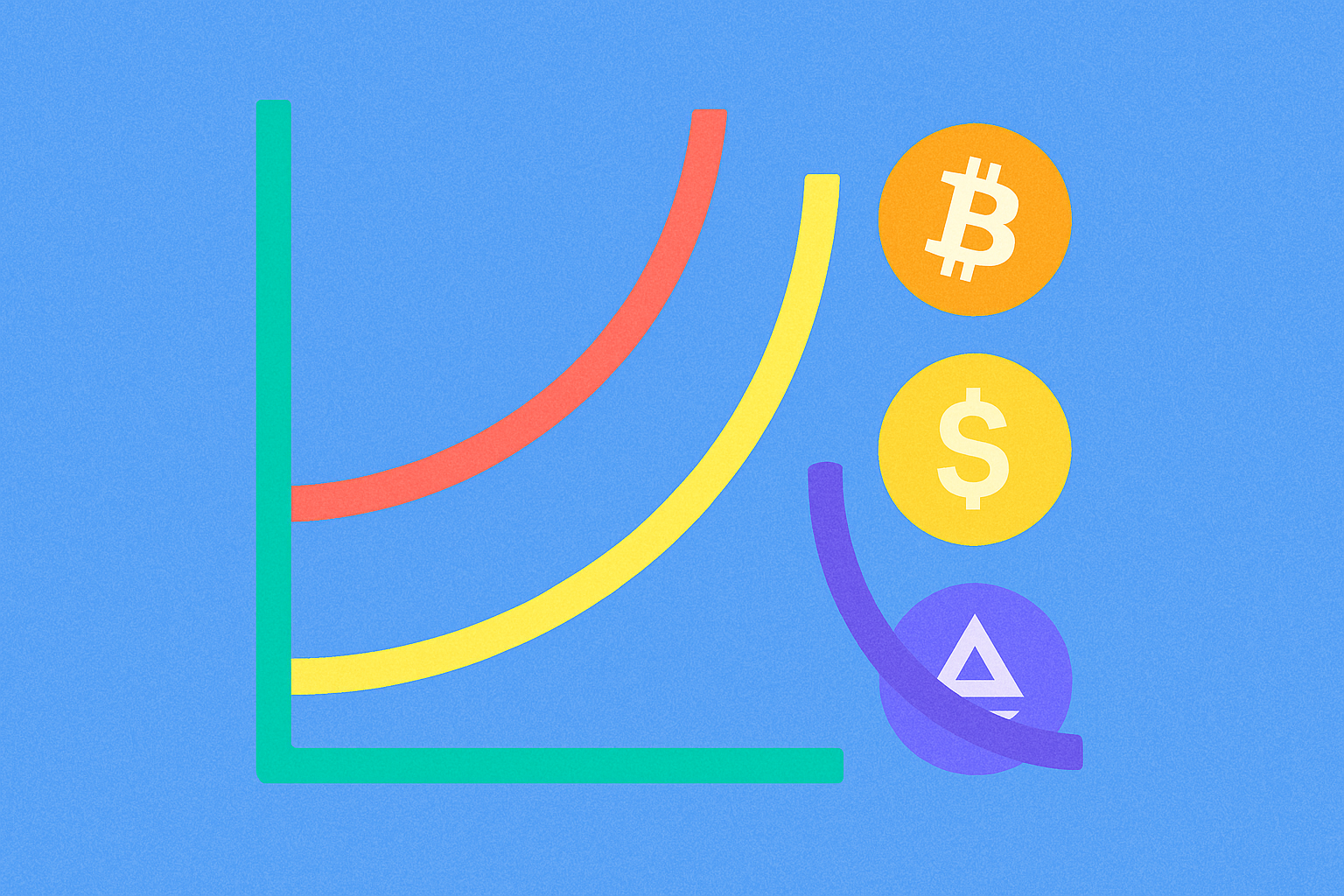
What Are the Types of Bonding Curves?

A linear bonding curve is perhaps the simplest to understand, but depending on what the developer wants to accomplish, they might want to encourage early investment or discourage early selling, among other strategic objectives. As a bonding curve is built into the blockchain and is typically unchangeable once deployed, the shape it takes will determine these aspects when investors buy and sell. The choice of curve shape is therefore a critical design decision that significantly impacts token economics.

There are four most commonly used bonding curves:

1. Sigmoid Curve
2. Quadratic Curve
3. Negative Exponential Curve
4. Linear Curve

Different bonding curve shapes will be adopted based on what type of investment behavior and growth pattern the developer is looking for:

To Reward Early Investors: If a developer wants to significantly reward early investors, they can use a sigmoid or quadratic bonding curve. These bonding curves are particularly effective for projects that a developer expects to experience viral growth or rapid adoption. These could be projects that are geared toward quite a large audience, for example a platform that revolves around blockchain gaming like GameFi ecosystems, a platform that creates and sells non-fungible tokens (NFTs) like ECOMI, or an audio sharing platform like Audius. Here, a developer could use a sigmoid curve to keep costs low for early investors while dramatically increasing the cost once reaching the more mainstream adopters. This can be seen by the sharp increase in price at the inflection point in the sigmoid curve, which creates a clear incentive structure. Alternatively, they could use a quadratic bonding curve to offer a steadier increase that is still significantly lower for early investors than latecomers, providing a more gradual but still substantial reward for early participation.

To Incentivize Early Investment but Not Disincentivize Later Investment: If a developer is using a bonding curve for a project that requires a long period of sustained investment, for example a fundraising project or a platform building long-term infrastructure, then they might use a negative exponential curve or a linear bonding curve. By using a negative exponential curve, the developer incentivizes the investor by giving them a chance to buy in at a low cost and make a profit on their investment during the early steep phase. As the project gathers more interest and more investment, the curve begins to flatten, finally having only a gradual increase. This ensures that later investors are not discouraged by prohibitively high prices. With a linear bonding curve, the developers will have a steady, predictable increase in cost as the project gathers more investors. A linear bonding curve is also more profitable for early investors due to the cumulative cost structure, but there is not such a large contrast between costs for early and late investors as with the sigmoid and quadratic curves, making it more equitable over time.

To Keep Costs Continuous and Stable: A linear bonding curve can also be used for projects where investors are not primarily looking to make or lose money from that investment, but rather to participate in a community or support a cause. Here, the cost remains steady and predictable, meaning minimal speculation and volatility. This type of bonding curve could work well for investors who are simply supporting a project that they believe in, such as community-driven initiatives or public goods funding, where the focus is on utility and participation rather than profit maximization.

Advantages of Bonding Curves

Bonding curves offer numerous compelling advantages that have made them increasingly popular in the cryptocurrency space:

1. Continuous Liquidity: Bonding curves provide a guaranteed price for buying or selling tokens directly from the smart contract, ensuring liquidity without the need for market makers or centralized exchanges. This means that participants can always enter or exit positions, regardless of trading volume or market conditions, eliminating the liquidity risk common in traditional markets.

2. Fair and Transparent Pricing: The pricing formula is public and predefined in the smart contract code, ensuring fairness as everyone faces the same conditions. This transparency builds trust among participants, as the logic is immutable on-chain and can be verified by anyone. There are no hidden fees or opaque pricing mechanisms that could disadvantage certain participants.

3. Bootstrap Funding: Bonding curves enable projects to fundraise effortlessly and continuously, automatically managing token sales without the need for complex ICO infrastructure or regulatory compliance burdens. This allows funding to align with actual interest over time, creating a more organic and sustainable growth pattern rather than the boom-and-bust cycles often seen with traditional token sales.

4. Incentivize Early Adoption: Early adopters benefit from lower prices in a structured and predictable way, fostering a supportive community that is invested in the project's long-term success. This creates natural ambassadors who have both financial and emotional incentives to promote the project, helping to drive organic growth and network effects.

5. Automatic Market Making: In DeFi applications, bonding curves facilitate automated exchanges without requiring order books or centralized intermediaries. This democratizes liquidity provision, allowing anyone to participate in market making, and reduces reliance on traditional market-making infrastructure that often favors institutional players.

6. Predictability for Token Economics: Projects can simulate various demand scenarios to estimate pricing trajectories and funding outcomes before launch. This provides a stable tokenomics framework that can reduce speculative volatility, as participants can model expected price movements based on adoption curves. This predictability helps both developers and investors make more informed decisions.

7. Aligning Value with Usage: Bonding curves can effectively link token value to system participation and utility, creating a virtuous cycle where increased participation raises token prices, which in turn rewards users and attracts more participants. This alignment of incentives helps ensure that token value reflects actual usage and utility rather than pure speculation.

Risks and Challenges of Bonding Curves

While bonding curves are powerful tools, they are not without limitations and come with their own set of risks and considerations that participants must understand:

1. Volatility and Speculation: Exponential bonding curves can lead to extreme price fluctuations, encouraging speculative behavior rather than genuine usage. Early holders might sell off tokens to realize profits, causing prices to drop sharply and harming later participants who bought at higher prices. This can create boom-and-bust cycles that undermine the project's stability and long-term viability.

2. Whale Manipulation: Large buyers or sellers can significantly impact prices on bonding curves due to the mathematical relationship between supply and price. A whale buying a large number of tokens can artificially inflate prices for later buyers, while a large sell-off can crash the price, making such curves particularly sensitive to large transactions. This concentration of power can disadvantage smaller participants and create unfair market conditions.

3. Liquidity vs. Price Impact: While bonding curves generally offer good liquidity in that you can always transact, larger trades can cause considerable price slippage, especially on steep curves or with smaller reserve pools. This means that the effective price paid for large purchases or received for large sales can differ significantly from the quoted price, creating execution risk for substantial transactions.

4. Smart Contract Risk: Bonding curves rely on complex smart contracts that must be carefully audited and tested. These contracts may contain vulnerabilities or bugs that could be exploited. A critical bug could allow unauthorized token minting without proper collateral exchange or compromise reserve assets, creating catastrophic losses for users. The immutable nature of blockchain means that bugs cannot be easily fixed once deployed.

5. Capital Inefficiency: Some bonding curve models lock significant funds as reserves for liquidity provision, leading to opportunity costs as this capital could potentially be deployed elsewhere. Mismanagement of reserves or insufficient reserve ratios can cause reserves to inadequately cover token supply, impacting user confidence and potentially leading to bank-run scenarios.

6. Complexity and User Understanding: Bonding curves can confuse users, particularly those unfamiliar with mathematical concepts or DeFi mechanisms. Users may overpay due to not understanding price impact, or panic sell if they don't understand how their actions affect prices. This complexity barrier can limit adoption and lead to poor user experiences, especially for less sophisticated participants.

7. Potential for Bank Run Dynamics: In cases of reduced confidence, especially in stablecoin or reserve-backed systems, a sudden rush to sell can lead to a cascading price crash if reserves are insufficient or if the curve is too steep. This creates systemic risk where fear becomes self-fulfilling, as seen in various algorithmic stablecoin failures.

8. Regulatory Considerations: Bonding curves could potentially be classified as securities offerings under certain jurisdictions, attracting regulatory scrutiny, particularly if tokens are bought with profit expectations rather than utility purposes. Compliance with securities laws is essential but can be complex and varies by jurisdiction, creating legal uncertainty for projects and participants.

9. Arbitrage and External Market Effects: If tokens trade on multiple platforms including both bonding curves and external exchanges, price discrepancies can arise, leading to arbitrage opportunities. While arbitrage can help align prices, it can also drain reserves from bonding curves or create unexpected volatility as traders exploit price differences between venues.

Conclusion

Bonding curves represent a sophisticated type of automated market maker (AMM) that uses algorithmic trading to calculate token value according to pre-established mathematical formulas and token supply dynamics. This means that an investor can buy tokens using collateral and then sell their tokens whenever they want, all directly through the smart contract without intermediaries. This approach reduces human error through automation and mathematical precision, creates a completely transparent trading process where all rules are visible on-chain, and maintains decentralization since everything is carried out through smart contracts without centralized control.

Bonding curves are a powerful way for developers to implement their own investment strategies and token economics in a transparent and error-free manner, without the need for centralized exchanges or traditional market makers. In addition, bonding curves can help investors predict how much their assets could rise in value based on projected adoption, and thus calculate their potential returns. It is important to note, however, that although a bonding curve can show how much an asset could theoretically rise based on supply dynamics, it cannot guarantee that the tokens will actually be bought, and thus it does not guarantee that the token will reach that projected value. Market demand remains the ultimate determinant of success.

In summary, bonding curves have proven to be a powerful and versatile concept for aligning incentives and enabling fluid, decentralized markets in the crypto space. They embody the core spirit of DeFi: removing middlemen and encoding financial logic directly on blockchain through transparent, immutable smart contracts. For users, the key takeaway is that bonding curves are fundamentally about the interplay of supply and demand coded into an algorithm, creating predictable price discovery mechanisms. If you participate in a token sale or DeFi protocol using bonding curves, understanding the specific curve shape and its implications—including both the opportunities and risks—will help you make informed decisions and navigate this innovative but complex mechanism effectively. As the cryptocurrency ecosystem continues to evolve, bonding curves will likely remain an important tool for creating sustainable token economies and decentralized markets.

FAQ

What is a bonding curve and what role does it play in cryptocurrency?

A bonding curve is a smart contract mechanism that dynamically adjusts token prices based on supply and demand. It calculates individual token prices according to circulating supply, ensuring liquidity and market stability while maintaining price balance in crypto ecosystems.

How does Bonding Curve determine token price? What is the mechanism of price changes with supply variations?

Bonding Curve uses a mathematical formula to automatically adjust token price based on supply changes. As supply increases, price rises; as supply decreases, price falls. This ensures fair, rule-based pricing determined by market demand dynamics.

What are some crypto projects using bonding curves? What do real examples look like?

Friend.Tech and Sidekick are notable examples using bonding curves. Friend.Tech combined private fan tokens with bonding curves for creator monetization, while Sidekick explores this model in social platforms. These projects demonstrate how bonding curves enable dynamic pricing and community engagement in crypto applications.

Bonding curve相比传统市场流动性机制有什么优势和劣势?

Bonding curve provides decentralized liquidity without market makers, but it can lead to less efficient price discovery and higher slippage compared to traditional market mechanisms.

What are the risks of investing in bonding curve tokens? What risk factors do I need to understand?

Bonding curve token risks include market volatility, dynamic pricing fluctuations, and project-specific risks. Token prices are non-fixed and can fluctuate significantly based on supply and demand. Investment does not guarantee returns or liquidity.

What does slippage in bonding curves mean and how is it calculated?

Slippage is the difference between expected execution price and actual transaction price. Calculate it as: Slippage = Expected Price - Actual Execution Price. It reflects market liquidity and transaction costs during bonding curve trades.